Supervised Tracking of Fiducial Markers in Magnetic Tweezer Measurements

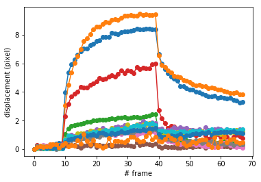
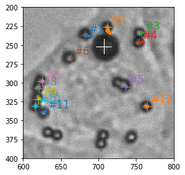
Left: the image of beads on cells loaded in ClickPoints. Right: displacement of beads.

In the example, we show how the ClickPoints addon Track can be used to track objects in an image and how the resulting tracks can later on be used to calculate displacements. [Bonakdar2016]

The data we show in this example are measurements of a magnetic tweezer, which uses a magnetic field to apply forces on cells. The cell is additionally tagged with non magnetic beads, with are used as fiducial markers.

The images can be opened with ClickPoints and every small bead (the fiducial markers) is marked with a marker of type tracks. Then the Track addon is started to finde the position of these beads in the subsequent images.

The resulting tracks can now be accessed and evaluated with Python and the ClickPoints package. Therefore we first open the ClickPoints file:

%matplotlib inline

import numpy as np
import matplotlib.pyplot as plt

# connect to ClickPoints database
# database filename is supplied as command line argument when started from ClickPoints
import clickpoints
db = clickpoints.DataFile("track.cdb")

path track.cdb
Open database with version 18

Then we get all the tracks with getTracks(). In this example without any filtering, as we just want all the tracks available. We can iterate ofer the received object and access the Track objects. From them we can get the points and calculate their displacements with respect to their staring points.

# get all tracks
tracks = db.getTracks()

# iterate over all tracks
for track in tracks:
    # get the points
    points = track.points
    # calculate the distance to the first point
    distance = np.linalg.norm(points[:, :] - points[0, :], axis=1)
    # plot the displacement
    plt.plot(track.frames, distance, "-o")

# label the axes
plt.xlabel("# frame")
plt.ylabel("displacement (pixel)")

<matplotlib.text.Text at 0x2b3f44019e8>

We can now use getImage() to get the first image of the sequence and load the data from this file. This can now be displayed with matplotlib. To draw the tracks, we itarate over the track list again and plot all the points, as well, as the starting point of the track for a visualisation of the tracks.

# get the first image
im_entry = db.getImage(0)

# we load the pixel data from the Image database entry
im_pixel = im_entry.data

# plot the image
plt.imshow(im_pixel, cmap="gray")

# iterate over all tracks
for track in tracks:
    # get the points
    points = track.points
    # plot the beginning of the track
    cross, = plt.plot(points[0, 0], points[0, 1], '+', ms=14, mew=1)
    # plot the track with the same color
    plt.plot(points[:, 0], points[:, 1], lw=3, color=cross.get_color())
    # plot the track id with a little offset and the same color
    plt.text(points[0, 0]+5, points[0, 1]-5, "#%d" % track.id, color=cross.get_color(), fontsize=15)

# zoom into the image
plt.xlim(600, 800)
plt.ylim(400, 200)

(400, 200)

References

Bonakdar2016

Navid Bonakdar, Richard Gerum, Michael Kuhn, Marina Spörrer, Anna Lippert, Werner Schneider, Katerina E Aifantis, and Ben Fabry. Mechanical plasticity of cells. Nature Materials, 2016.