Using ClickPoints for Visualizing Simulation Results

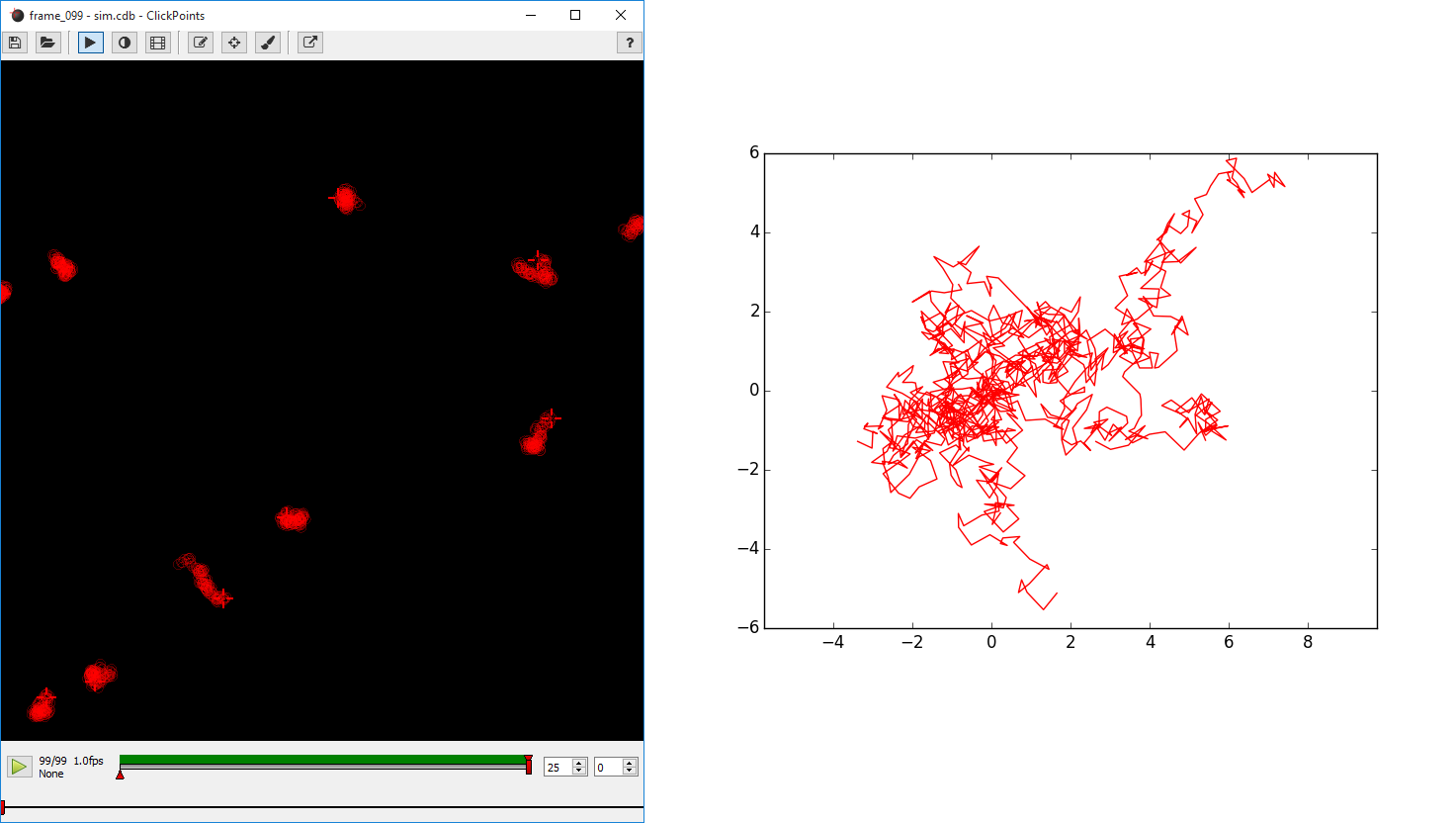
Left: Tracks of the random walk simulation in ClickPoints. Right: Tracks plotted all starting from (0, 0).

Here we show how ClickPoints can be apart from viewing and analyzing images also be used to store simulation results in a ClickPoints Project file. This has the advantages that the simulation can later be viewed in ClickPoints, with all the features of playback, zooming and panning. Also the coordinates of the objects used in the simulation can later be accessed through the ClickPoints database file.

This simple example simulates the movement of 10 object which follow a random walk.

First some imports:

%matplotlib inline
import matplotlib.pyplot as plt
import numpy as np
import clickpoints

Then we define the basic parameters for the simulation.

# Simulation parameters
N = 10
size = 100
size = 100
frame_count = 100

We create a new database. The attribute “w” stands for write, which ensures that we create a new database.

# create new database
db = clickpoints.DataFile("sim.cdb", "w")

path sim.cdb

We define a new marker type with the name “point” the color red (“#FF0000”) and the type TYPE_Track. Then we create N track instances for it.

# Create a new marker type
type_point = db.setMarkerType("point", "#FF0000", mode=db.TYPE_Track)

# Create track instances
tracks = [db.setTrack(type_point) for i in range(N)]

We create some random initial positions for the tracks. We now iterate over the amout if frames we want to simulate. For each iteration we add a new image to the database using setImage(), then we add some random movement to the positions and store the new positions for the tracks using setMarkers(). Here we have to provide the current image and the list of Track objects.

# Fix the seed
np.random.seed(0)

# Create initial positions
points = np.random.rand(N, 2)*size

# iterate
for i in range(frame_count):
    # Create a new frame
    image = db.setImage("frame_%03d" % i, width=size, height=size)

    # Move the positions
    points += np.random.rand(N, 2)-0.5

    # Save the new positions
    db.setMarkers(image=image, x=points[:, 0], y=points[:, 1], track=tracks)

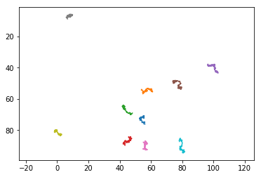
After the simulation, we want to access the tracks again to plot them. From every track we query the points and plot them.

# plot the results
for track in tracks:
    plt.plot(track.points[:, 0], track.points[:, 1], '-')
# adjust the plot ranges
plt.xlim(0, size)
plt.ylim(size, 0)
# and adjust the scaling to equal
plt.axis("equal")
plt.show()

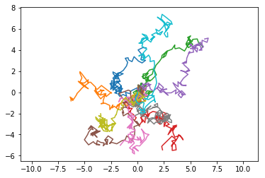
We now plot the tracks in a different fashion, as a “rose” plot, where all the tracks start at the same position.

# plot the results
for track in tracks:
    # get the points
    points = track.points
    # substract the inital point
    points = points-points[0, :]
    # plot the track from the new origin
    plt.plot(points[:, 0], points[:, 1], '-')
# and adjust the scaling to equal
plt.axis("equal")
plt.show()