Flourescence intensities in plant roots

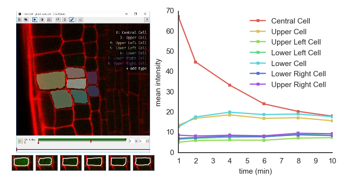
Left: image of a plant root in ClickPoints. Right: fluorescence intensities of the cells over time.

In the example, we show how the mask panting feature of ClickPoints can be used to evaluate fluorescence intensities in microscope recordings.

Images of an Arabidopsis thaliana root tip, obtained using a two-photon confocal microscope [Gerlitz2016], recorded at 1 min time intervals are used. The plant roots expressed a photoactivatable green fluorescent protein, which after activation with a UV pulse diffuses from the activated cells to the neighbouring cells.

For each time step a mask is painted to cover each cell in each time step.

The fluorescence intensities be evaluated using a python script.

Open the the database where the masks are painted:

import re
import numpy as np
from matplotlib import pyplot as plt
import clickpoints

# open the ClickPoints database
db = clickpoints.DataFile("plant_root.cdb")

path plant_root.cdb
Open database with version 18

Get a list of Image objects (getImages()) and a list of all MaskType objects (getMaskTypes()). Then we iterate over the images, load the green channel of the image (image.data[:, :, 1]) and get the mask data for that image (image.mask.data). The mask data is a numpy array with the same dimensions as the image having 0s for the background and the value mask_type.index for each pixel that belongs to the mask_type. Therefore we iterate over all the mask types and filter the pixels of the mask that belong to each type. This mask can then be used to filter the pixels of the green channel that belong to the MaskType.

# get images and mask_types
images = db.getImages()
mask_types = db.getMaskTypes()

# regular expression to get time from filename
regex = re.compile(r".*(?P<experiment>\d*)-(?P<time>\d*)min")

# initialize arrays for times and intensities
times = []
intensities = []

# iterate over all images
for image in images:
    print("Image", image.filename)
    # get time from filename
    time = float(regex.match(image.filename).groupdict()["time"])
    times.append(time)

    # get mask and green channel of image
    mask = image.mask.data
    green_channel = image.data[:, :, 1]

    # iterate over the mask types
    intensity = []
    for mask_type in mask_types:
        # filter from the mask the current mask type
        mask_for_this_type = (mask == mask_type.index)
        # calculate the mean intenstiry of this cell in the green channel
        mean_intensitry_in_cell = np.mean(green_channel[mask_for_this_type])
        # and add it to the list
        intensity.append(mean_intensitry_in_cell)
    # add all the mean intensities of the cells in this image to a list
    intensities.append(intensity)

Image 1-0min.tif
Image 1-2min.tif
Image 1-4min.tif
Image 1-6min.tif
Image 1-8min.tif
Image 1-10min.tif

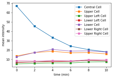
We now plot the intensitry for each cell over the time. The label of each line is the name of the corresponding MaskType.

# convert lists to numpy arrays
intensities = np.array(intensities).T
times = np.array(times)

# iterate over cells
for mask_type, cell_int in zip(mask_types, intensities):
    plt.plot(times, cell_int, "-s", label=mask_type.name)

# add legend and labels
plt.legend()
plt.xlabel("time (min)")
plt.ylabel("mean intensity")
# display the plot
plt.show()

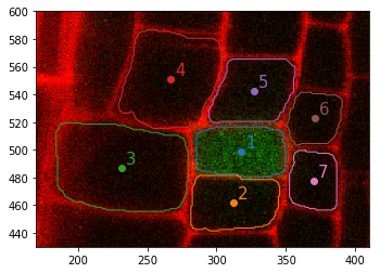
How we want to visualize the cells in the image. Therefore we fetch the first image and its mask. Then we iterate over all mask types and draw countours around each masked region. Then we plot the centroid of the mask and the mask index.

from skimage.measure import regionprops, label, find_contours

# get the first image
image = db.getImage(0)
# get the corresponding mask data
mask_data = image.mask.data
# iterate over all mask types
for mask_type in mask_types:
    # get the mask data for that mask type
    mask = (mask_data == mask_type.index)

    # get the contour of the masked region and draw it
    contour = find_contours(mask, 0.5)[0]
    line, = plt.plot(contour[:, 1], contour[:, 0], '-', lw=1)

    # get the centroid and draw a dot with the same color
    prop = regionprops(label(mask))[0]
    y, x = prop.centroid
    plt.plot(x, y, 'o', color=line.get_color())
    # and a text showing the index of the mask type with the same color
    plt.text(x+3, y+3, '%d' % mask_type.index, color=line.get_color(), fontsize=15)
# draw the image
plt.imshow(image.data)
# and zoom in
plt.xlim(170, 410)
plt.ylim(430, 600)
plt.show()

References

Gerlitz2016

Nadja Gerlitz. Dronpa. 2016.